Creating Generative Geometric Art in Python

The Challenge

I am a firm believer that anything and everything you learn can shape your life in the most unexpected way. Thinking “out-of-the-box” is usually just applying what you have learnt in a seemingly unrelated domain to the problem at hand.

The problem was simple, I had to design digital art for glass doors to be installed in my living room to match the abstract art painted on one of its walls. Initially, I was distracted by the standard tools for the job, digital art tools such as Krita or INKSCAPE. But frustrated by the amount of time needed to learn digital art as someone with no experience, I was motivated to think outside the box. And then I had a flash of inspiration: the python library plotly is capable of generating SVG files and an abstract triangular pattern is nothing more than a randomly seeded triangular mesh.

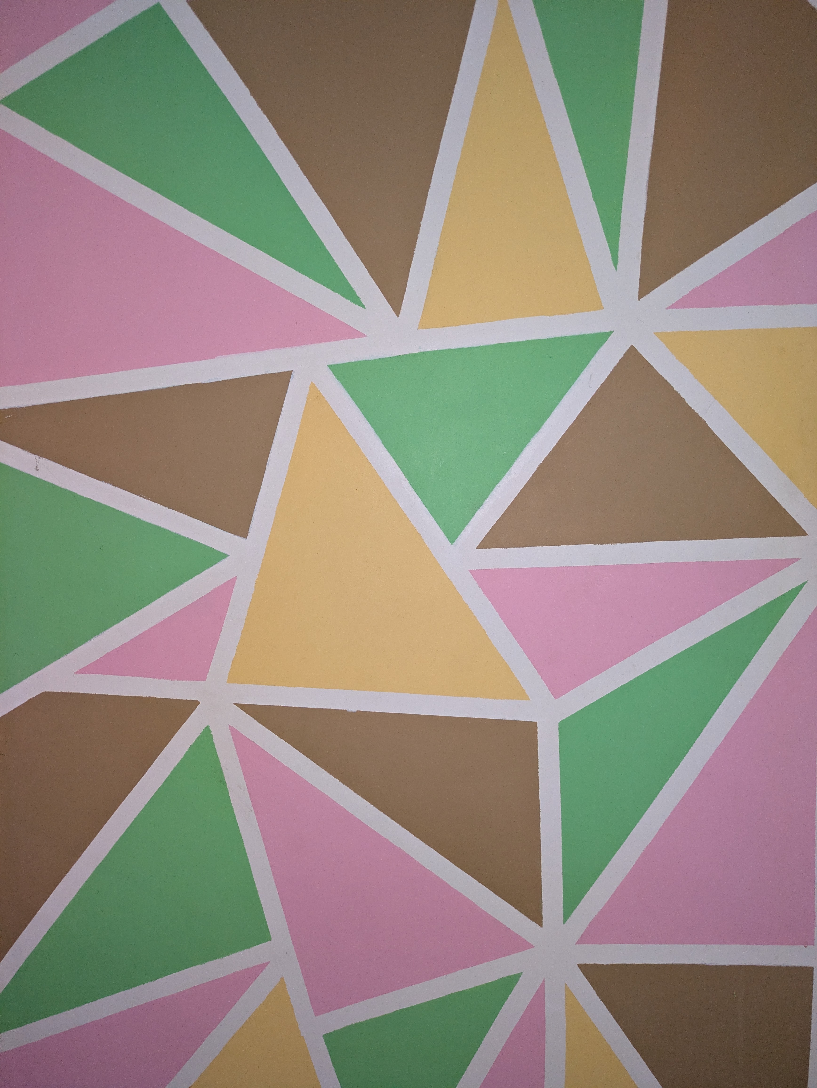
I have always been drawn to the idea of Creative Programming, having been introduced to it by the creativecoding subreddit. This was the perfect opportunity to try my hand it, without falling into the rabbit hole of exploring mathematics and computer science way beyond what I already know.

The Solution

Delaunay Triangulation

Delaunay triangulation is a method to generate triangles in a given space while avoiding “sliver triangle” i.e. triangles with at least one of the interior angles being very small. This is achieved mathematically by generating a set of points such that the circumcircle of any triangle does not contain any points other than the three points of the triangle, hence ensuring that the minimum interior angles of the triangles are maximised and slivers are avoided.

Delaunay triangulation is widely used in mesh generation algorithms in FEA. This is because the geometry of sliver triangles doesn’t work very well with FEA formulations and their presence brings down the quality of the solution. Because of its widespread use in meshing, implementation of the Delaunay triangulation algorithm is readily available in the scipy package, making the initial implementation easy.

The first version of the script is pretty simple and straightforward. A set of random points are generated, triangulated and plotted with plotly. Unfortunately, plotly doesn’t provide shape primitives for polygons other than rectangles, so the triangles are drawn using scatter traces as suggested in plotly docs. The triangles are coloured with the hex representation of the 4 colours on my wall, taken from the website of the paint manufacturer.

1
2
3
4
5
6
7
8
9
10
11
12
13
14
15
16
17
18
19
20
21
22
23
24
25
26
27
28
29
30
31
32
33
34
35
36
37
38
39
40
41
42
43
44
45
46
47
48
49
50
51
52
 
import numpy as np
from scipy.spatial import Delaunay
import plotly.graph_objects as go

def main():

    # 1. Random points
    pts = np.random.rand(200, 2)

    # 2. Delaunay triangulation
    tri = Delaunay(pts)

    # 4 colours to choose from
    palette = ["#fece8b", "#b49370", "#95CC84", "#f7b4c3"]

    fig = go.Figure()

    # For each triangle
    for simplex in tri.simplices:
        vertices = pts[simplex]
        x = vertices[:, 0]
        y = vertices[:, 1]

        # close the polygon
        x = np.append(x, x[0])
        y = np.append(y, y[0])

        fig.add_trace(go.Scatter(
            x=x,
            y=y,
            fill="toself",
            mode="lines",
            line=dict(color="white", width=6),
            fillcolor=np.random.choice(palette)
        ))

    fig.update_layout(
        showlegend=False,
        xaxis=dict(visible=False),
        yaxis=dict(visible=False),
        margin=dict(l=0, r=0, t=0, b=0),
        plot_bgcolor="white",
        paper_bgcolor="white"
    )
    _ = fig.update_xaxes(range=[0, 1])
    _ = fig.update_yaxes(range=[0, 1])

    fig.write_image("triangulation.svg")
    fig.write_image("triangulation.png")

if **name** == "**main**":
main()
 

This creates a simple Delaunay triangulation over the 2D space and colours them randomly. However, as seen in the following image, the points are generated completely randomly so there is no guarantee that the edges will be completely covered.

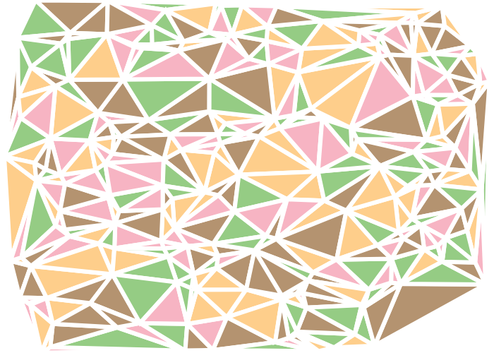
The solution for fixing the edges is quite simple, the triangulation just needs to be done for a larger region than the domain of the image. This will generate very natural looking edges as plotly does not clip the triangles and generates a clean edge.

# For example, change the image domain to:
_ = fig.update_xaxes(range=[0.33,0.66])
_ = fig.update_yaxes(range=[0.33,0.66])

Colour Clumping

A not so simple issue to solve is colour clumping which might occur through random colour distribution. Neighbouring triangles can be allocated the same colour which can lead to clumps of the same colour forming.

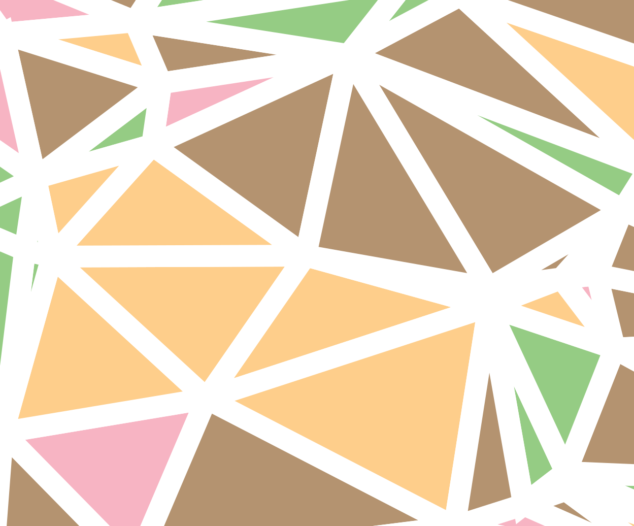
To avoid this, an adjacency list needs to be created. This is a two dimensional vector where each row corresponds to a list of triangles that neighbour it, i.e. share an edge with it. The most efficient way to create this is to create a map of edges and triangles. We simply loop through all triangles and check all edges; if the edge already exists in the map, both triangles are marked as neighbours, else the edge is just added to the map for future comparisons. Once the adjacency matrix is created, we can just ensure that a triangle is never allotted the same colour as its adjacent triangles.

palette = ["#fece8b", "#b49370", "#95CC84", "#f7b4c3"]
triangle_colours = [None] * len(tri.simplices)
adj = [[] for _ in tri.simplices]
edges = {}

for i, s in enumerate(tri.simplices):
for a, b in [(s[0], s[1]), (s[1], s[2]), (s[2], s[0])]:
key = tuple(sorted((a, b)))
if key in edges:
j = edges[key]
adj[i].append(j)
adj[j].append(i)
else:
edges[key] = i

# Assign colours with anti-clumping

for i in range(len(tri.simplices)):
neighbors = adj[i]
disallowed = {
triangle_colours[n] for n in neighbors if triangle_colours[n] is not None
}

    # Retry random colours until one fits
    for _ in range(10):
        c = np.random.choice(palette)
        if c not in disallowed:
            triangle_colours[i] = c
            break
    else:
        # fallback
        triangle_colours[i] = np.random.choice(palette)

Poisson-Disc Sampling

Another significant issue with the initial script is that the distribution of the points is uneven, which creates triangles of very different sizes which is not visually pleasing.

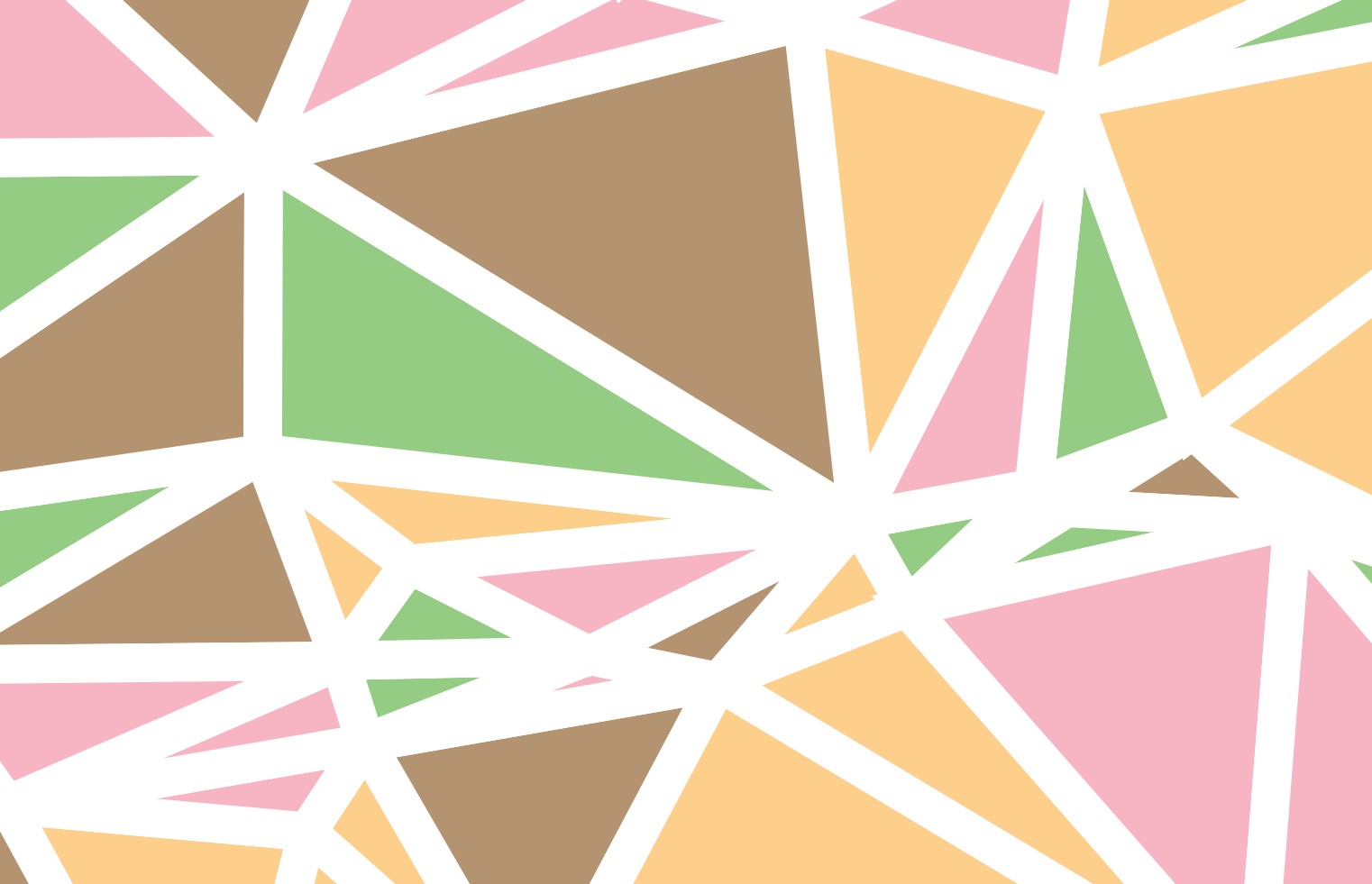
The solution for this is to use Poisson-Disc sampling, which is a method to sample points in space with a defined minimum separation instead of purely random sampling. Poisson-Disc is a very well studied method and the Bridson’s algorithm can generate them in $O(n)$ time. Unfortunately, the known python implementation of this algorithm poisson-disc is severely outdated and doesn’t work with recent versions of numpy. Hence, I ended up creating a very simple implementation of the algorithm myself.

def poisson_disc_samples(width, height, r, k=30):
"""
Bridson's Poisson-disc sampling algorithm.

    width, height : sampling area
    r             : minimum distance between samples
    k             : number of candidate attempts per active point
    """
    cell_size = r / np.sqrt(2)
    grid_width = int(np.ceil(width / cell_size))
    grid_height = int(np.ceil(height / cell_size))

    # Grid to store sample indices (-1 means empty)
    grid = -np.ones((grid_height, grid_width), dtype=int)

    samples = []
    active = []

    # Start with a random point
    p = np.array([np.random.uniform(0, width), np.random.uniform(0, height)])
    samples.append(p)
    active.append(0)

    gx = int(p[0] // cell_size)
    gy = int(p[1] // cell_size)
    grid[gy, gx] = 0

    while active:
        idx = np.random.choice(active)
        base = samples[idx]
        found = False

        # Try k random points around `base`
        for _ in range(k):
            theta = np.random.uniform(0, 2 * np.pi)
            rad = np.random.uniform(r, 2 * r)
            candidate = base + rad * np.array([np.cos(theta), np.sin(theta)])

            # Discard if outside the domain
            if not (0 <= candidate[0] < width and 0 <= candidate[1] < height):
                continue

            # Check neighbouring cells for conflicts
            cgx = int(candidate[0] // cell_size)
            cgy = int(candidate[1] // cell_size)

            ok = True
            for yy in range(max(0, cgy - 2), min(grid_height, cgy + 3)):
                for xx in range(max(0, cgx - 2), min(grid_width, cgx + 3)):
                    si = grid[yy, xx]
                    if si != -1:
                        if np.linalg.norm(samples[si] - candidate) < r:
                            ok = False
                            break
                if not ok:
                    break

            if ok:
                samples.append(candidate)
                active.append(len(samples) - 1)
                grid[cgy, cgx] = len(samples) - 1
                found = True
                break

        if not found:
            active.remove(idx)

    return np.array(samples)

The Results

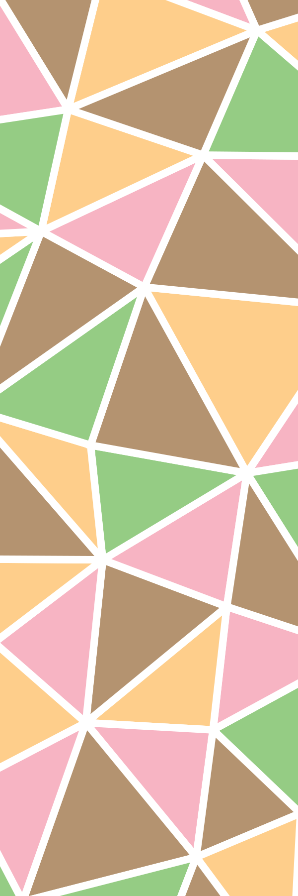
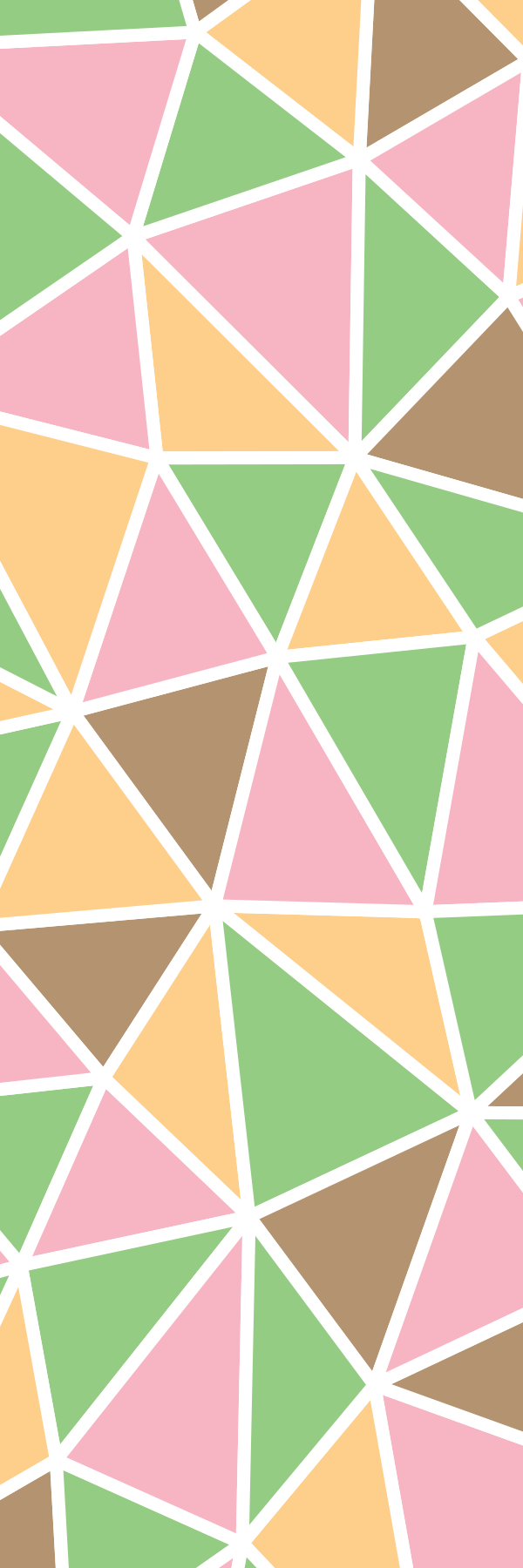
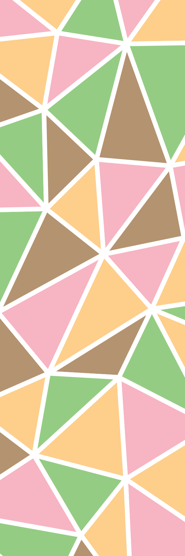
After putting everything together and refactoring the code to make it more modular, I was able to generate a set of images and picked the ones that I liked. The full code is available on GitHub.

This project reminded me that the numerical tools we use in engineering and simulation are often directly applicable to creative expression. The boundary between computational geometry and digital art is far thinner than we imagine.